Abstract

For the past couple of years, toy models have been extensively studied in the field of mechanistic interpretability. The concept of superposition, feature geometry, and how correlated/anticorrelated/uncorrelated features arrange themselves in these situations was first studied in Toy Models itself. This is my attempt to explain the theoretical foundation on why feature geometry in the infinite data regime for a ReLU model (with hidden=2) caps at a Pentagon geometry irrespective of the number of inputs. Additionally, I analyze the deviations to hexagon geometry as well, primarily analyzing two factors, i.e., initialization and the choice of optimizer, and their impact on feature geometry.

Introduction

The ReLU output model is a toy model replication of a neural network showcasing the mapping of features (5 input features) to hidden dimensions (2 hidden dimensions) where superposition can be introduced by changing the sparsity of input features. For a set of input features $x∈R^n$ and a hidden layer vector $h∈R^m$, where $n»m$, the model is defined as follows:

\[h=Wx\] \[x^′=ReLU(W^{T}h+b)\]

This model showcases how a large set of input features can be represented in a much smaller dimensional vector in a state of superposition by increasing the sparsity of the input features (sparsity tries to replicate the real-world data distribution where certain concepts are sparsely present throughout the training set). This concept and observations were first introduced in Anthropic’s Toy Models of Superposition paper

The original experiment was done on $n=5$ input features but when I try to increase the number of input features, an interesting phenomena occurs. Given the observations of a quadrilateral with $n=4$ and a pentagon with $n=5$, as the number of features increases one would expect feature geometry to be hexagon or heptagon, but in reality, the features restrict themselves to a pentagon geometry, with balance of the features (if they are learned by the model), overlapping with the existing 5 directions as shown in the figure below.

I wanted to understand in detail why this is the case and if it can help us improve our understanding of feature geometry in neural networks.

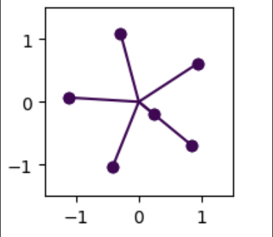
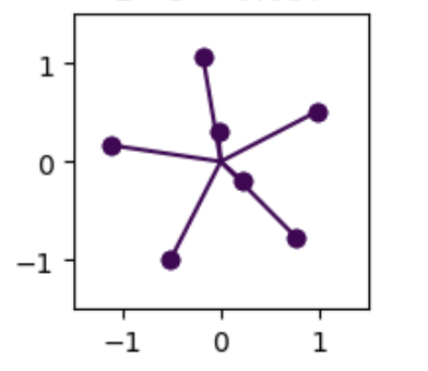
Fig.1 n_features = 6 (left) and 7 (right)

Relevance to AI Safety

One of the biggest subfields of AI safety is Mechanistic Interpretability. In this subfield, researchers try to reverse-engineer neural network models (which are considered black boxes as their internal mechanisms are unknown) and make them more interpretable. Toy model setup is a very important part of this subfield, as it allows us to do controlled experiments and understand the impact of different factors on different phenomena.

For example, the concept of superposition was first studied in Toy models of Superposition paper, which led to the creation of Sparse AutoEncoders (SAEs). Today, SAEs are an integral part of understanding the types of features a model is learning.

By understanding feature geometries in toy models, we aim to develop a strong intuition about how and when features are arranged in different geometries and the types of mechanisms governing a given geometry.

Different Data Regimes and Types of Features

Before diving deep into feature geometry and the experiments, I would like to explain the concept of data regimes because that majorly impacts the type of features the model learns.

The amount of data used to train the model has a massive impact on the types of features the model learns. Superposition, Memorization, and Double Descent showcase the impact of data regimes and how the model memorizes the dataset as features in low data regimes but transitions to learning generalizable features as the amount of data increases.

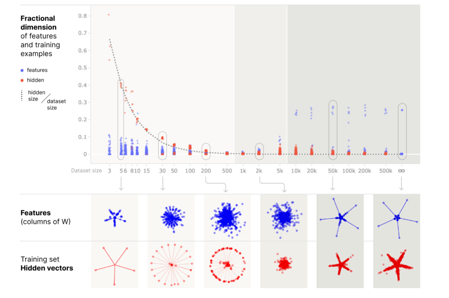
Fig.2 Increase in the data size leads to features transitioning from data features to generalizing features and the geometry converges to a pentagon. Source: https://transformer-circuits.pub/2023/toy-double-descent/index.html

I’ll be focusing on the infinite data regimes as it represents the closest condition to real-world models due to the sheer size of the datasets they are trained on. With the increase in data size, the feature geometry transitions towards the pentagon geometry, while in lower data regimes, the number of features represented was much higher due to the model memorizing the dataset.

Theoretical Intuition behind Pentagon Geometry

For building the theoretical intuition for why pentagon geometry is preferred by models, I’ll be walking you through this notebook shared by Anthropic. (Credits to Tom Henighan for open-sourcing this explanation)

The key factors governing the feature geometry is the balance between the overall loss of ignored features and the loss of represented features, along with the number of features that are ignored vs represented.

The expected loss due to ignoring a single feature can be defined as:

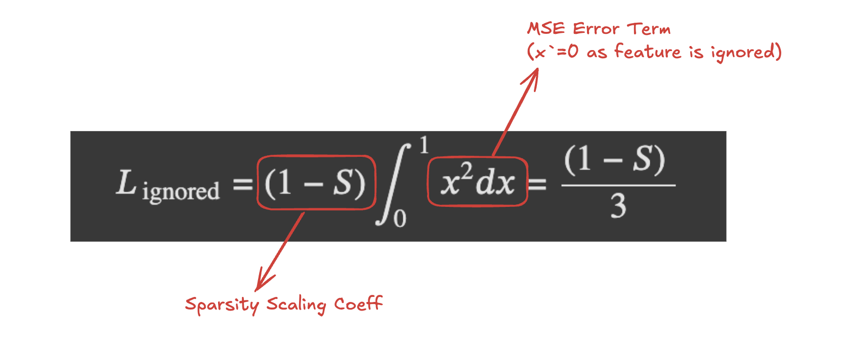
Fig.3 Expected loss due to ignoring a single feature

Note: A sparse regime is consiered for this scenario, as only sparse features are represented in superposition and $S$ represents the probability of $x_i$ being 0 otherwise it takes a value uniformly sampled between 0 and 1.

While the predicted value of $x_i’$ (when the feature is not ignored) can be defined by:

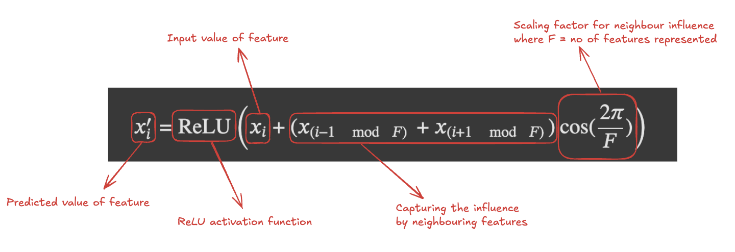
Fig.4 Predicted value when the feature is not ignored

The formula represents the predicted value in the form of the original input value and then bakes in the influence of nearest neighbouring features (if it is positive interference or negative interference). $mod F$ term helps us wrap around the features around every $F$ positions and $(i \pm 1 \mod F)$ refer to the nearest neighbours represented feature index.

After putting the above predicted term formula in the MSE loss formula, the loss due to the represented features can be defined by:

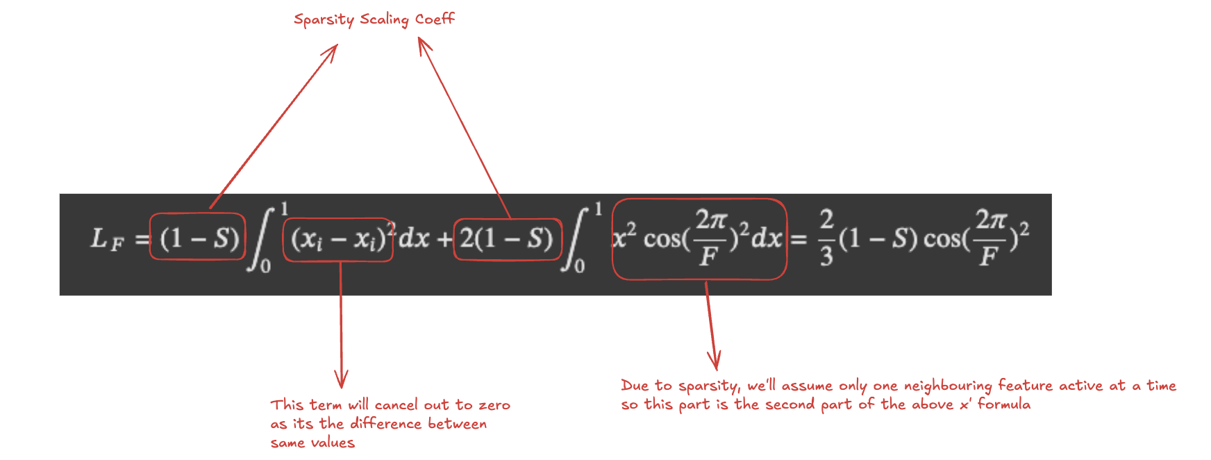
Fig.5 Loss due to the represented features

Currently, there are two Loss terms, and based on number of features represented, these two loss terms will be pulling the overall loss in opposite directions. Loss due to represented features will increase with the increase in the number of represented features due to increased interference from neighbouring features, but we want to avoid the Loss due to ignored features as well. So, the final entity to be minimised is the difference between $L_F$ and $L_{\text{ignored}}$ i.e.

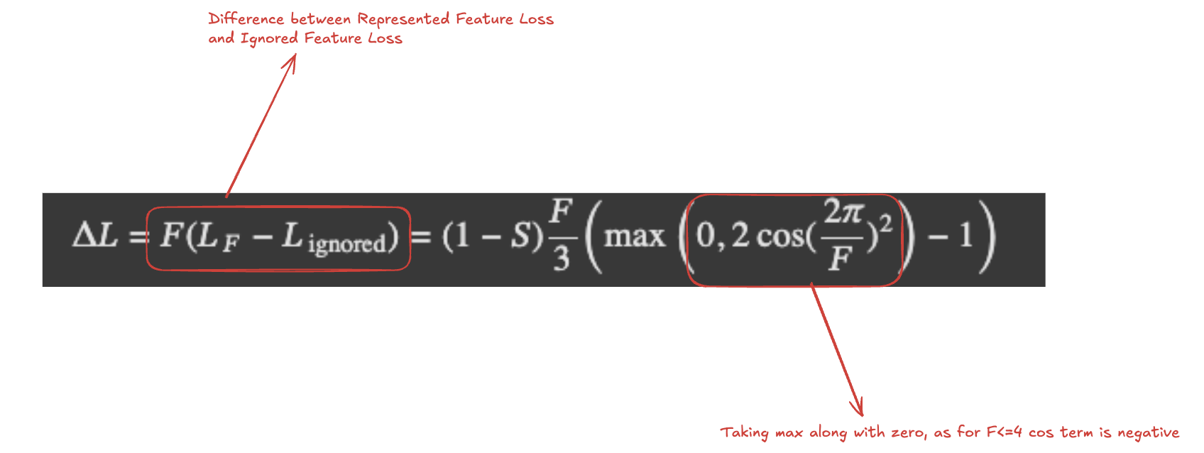
Fig.6 Difference between $L_F$ and $L_{\text{ignored}}$

After optimizing for $\Delta L$, the optimal point of lowest loss is reached at $F=5$.

The above derivation makes some assumptions for simplification and due to that the pentagon geometry is not always followed. There are some instances when a hexagon geometry (as shown in Fig 6) is observed as well. I’ll be conducting experiments to understand more about why this geometry was observed, what factors govern it and what is fundamentally different about hexagon geometry w.r.t pentagon geometry.

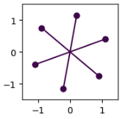
Fig.7 Hexagon Geometry in Toy models

Experiments

My experiment setup is similar to the Anthropic’s Toy models of Superposition setup with some modifications of my own. The number of input features will be 6 and all of them will have equal feature importance. I’ll be considering a sparsity value of 0.057 (as this sparsity was low enough to exhibit superposition but not low enough that features are not getting learned due to data unavailability) and will be analysing the effects of Initialization and the choice of Optimizer on hexagon feature geometry and superposition in general.

Impact of Initialization

While iterating the experiments through multiple different seeds, there are multiple instances where the final geometry is a hexagon while others are a pentagon. Following are the lists of experiments I performed to understand this behaviour

Feature Norms

At the start, when I compare the feature norms, there is a striking difference in the first glance itself. The overall norm in the hexagon geometry crosses the theoretical limit of $\sqrt{5}$ and stretches to 3 while the one for pentagon plateaus at 2.5.

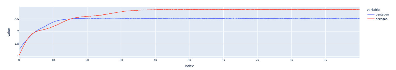
Fig.8 Feature Norms Pentagon vs Hexagon

Per Feature Gradient Norms and Losses

As a next step, I analyzed the trajectory of the per-feature gradient norm (to understand the types of gradient updates taking place) and compared it with per-feature loss to learn how the features are being learned.

In the case of pentagon geometry, the gradient updates for two features (dark blue and red) start at a very low point and stay low throughout the training run while for others it decreases in the later stages of the training process.

When compared against the per-feature losses, I observe that one feature is starting from a point of very low loss (very near to the optimal point) so it doesn’t need big gradient updates, but the other one is starting from a very high loss (very far from the optimal point) and still has low gradient updates indicating that its stuck in a saddle point and is unable to escape.

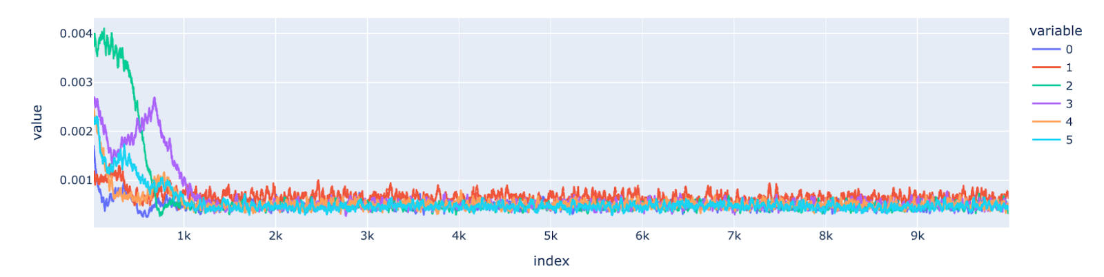
Fig.9 Per Feature Gradient Norm for Pentagon Seed

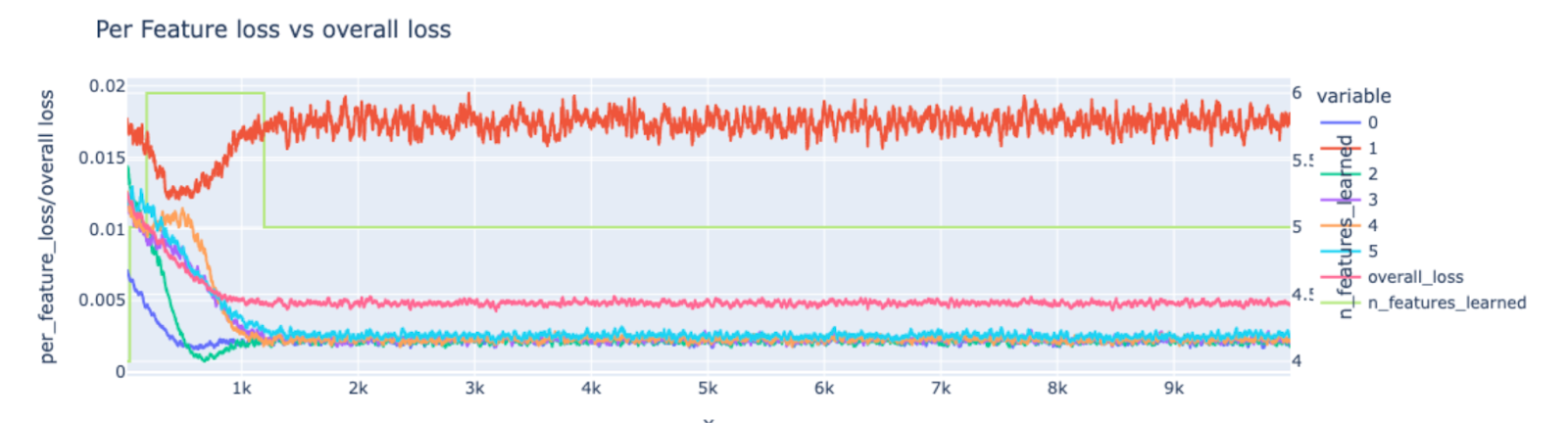
Fig.10 Per Feature Loss for Pentagon Seed

In the similar plots for hexagon geometry, it shows that the gradient updates decreases for all the features and the losses for all the features converge to a optimal minima as well.

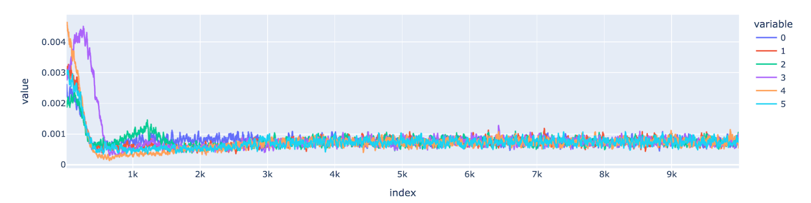
Fig.11 Per Feature Gradient Norm for Hexagon Seed

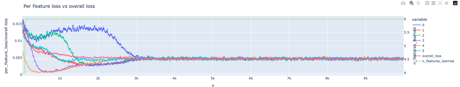
Fig.12 Per Feature Loss for Hexagon Seed

This analysis indicates the effect of initialization on the starting point of features in the coordinate space and how it affects the resulting feature geometry. To properly validate the hypothesis, I performed one more experiment of patching the initialization.

Hexagon Patching

I took the initial weights of the pentagon seed and replaced the weights of only the feature that is not learnt with initialization weights of the same feature from the hexagon seed. When the model is trained with this modified initial weight matrix, the resulting geometry showcases features arranged in a hexagon geometry after weight patching v/s in a pentagon geometry before patching.

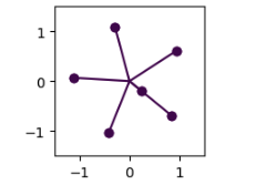
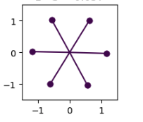
Fig.13 Unpatched Pentagon Geometry (left) and Patched Hexagon Geometry (right)

Impact of Optimizer

Secondly, I try to analyze the impact of the optimizer on the feature geometry. In this experiment, I chose 4 types of optimizers namely SGD, RMSProp, Adam, and AdamW.

In the experiments, SGD underperformed in all cases leading to non-superimposed and unlearned features irrespective of hyperparameters. For RMSProp, Adam & AdamW, all of them exhibit superposition and the resulting feature geometry was a delicate balance between initialization and choice of optimizer. Not all optimizers will give hexagon geometries at the same seed but once carefully chosen, the combination of the right seed and right optimizer will lead to the hexagon geometry, otherwise, it exhibits pentagon geometry.

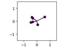
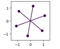
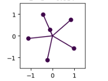
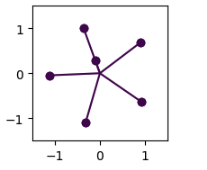
Fig.14 SGD (first), Adam (Second), AdamW (Third), RMSProp (Fourth)

Conclusion

In this analysis, I try to understand the core intuition behind the feature geometry in toy models with hidden dimension=2 and assumptions behind it. I also try to understand in what cases the experimental results deviate from the theoretical foundation leading to a hexagonal geometry and analyse the impact of Initialization and Optimizer on the resulting feature geometry.

Limitations and Future Work

While I found some pretty interesting results, there is still a much deeper analysis which can be conducted to study hexagon geometry and why it occurs. Also, this analysis was done on toy models so will the findings scale to bigger models or not, thats yet to be seen.

Acknowledgement

I want to thank Bluedot Impact for organizing the AISF Alignment Cohort. Past 12 weeks have been really valuable in improving my understanding on Mechanistic Interpretability and AI Safety in general.

Additionally, I want to thank Shivam Raval for guiding me through the research process.

About Me

Hey, I’m Shreyans and I’m an Independent Interpretability Researcher based out of Bengaluru, India. After 8 years of working in the Applied ML field, I finally took the leap of faith to take a small career break to pursue my interest of Interpretability Research. This work is my capstone project as part of the AISF Alignment Cohort by Bluedot Impact. If you have any questions or feedback on this blog, feel free to reach out to me on jshrey8@gmail.com or any of my socials in my profile. I hope I was able to improve your understanding on feature geometry in toy models. Cheers!!