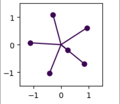
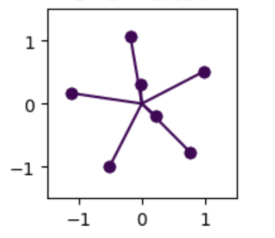
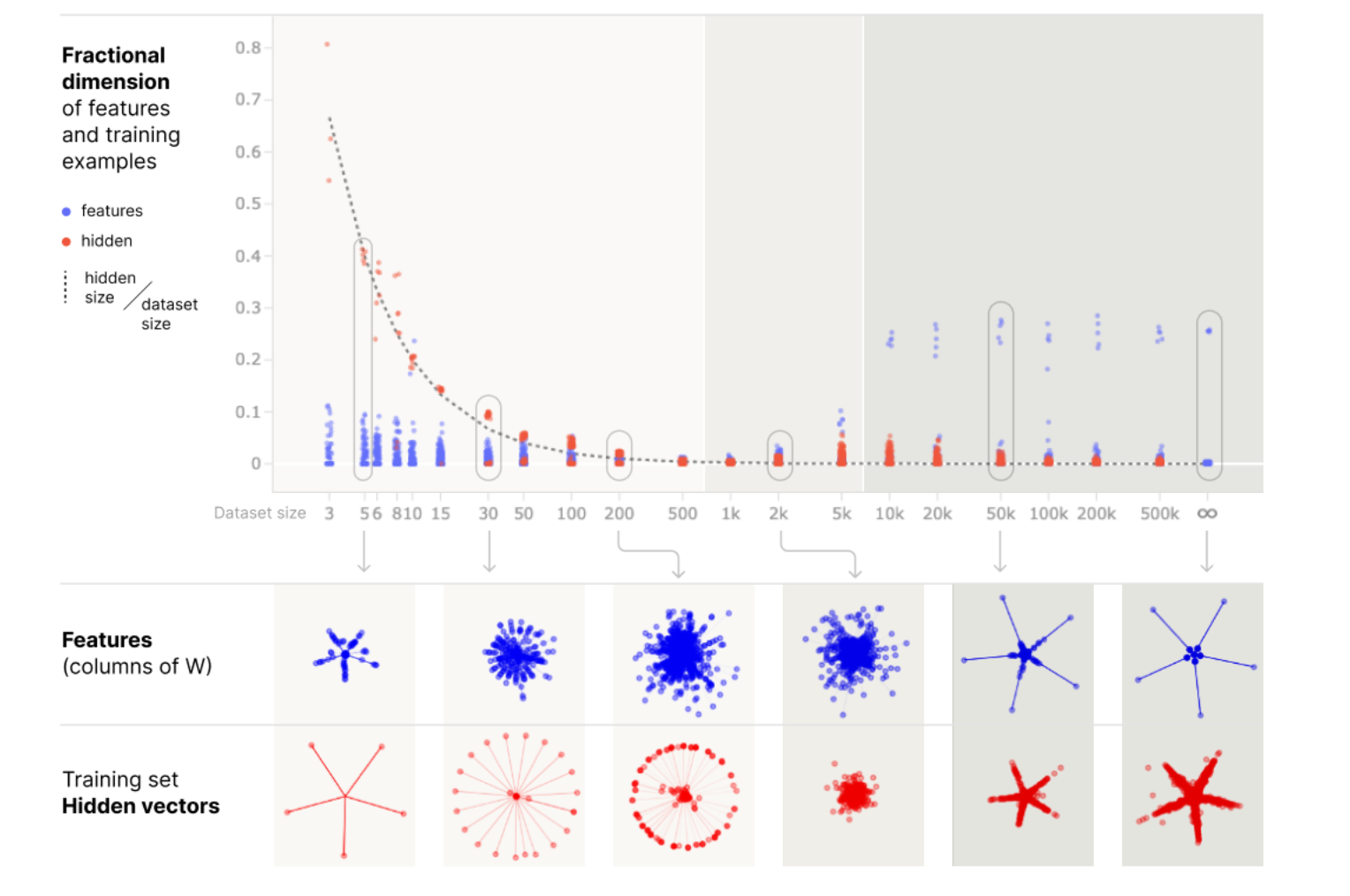
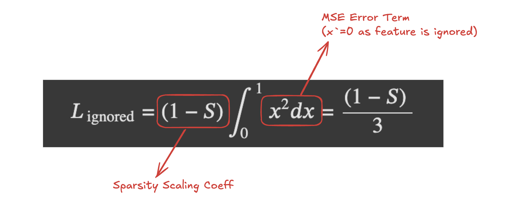
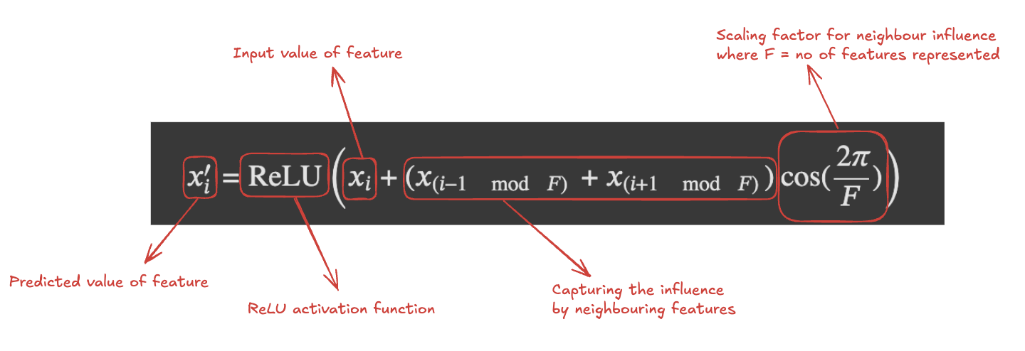
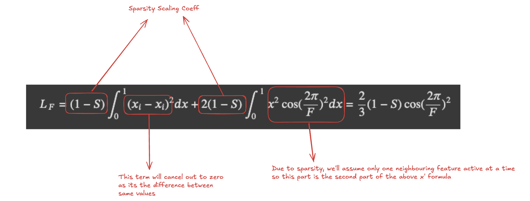
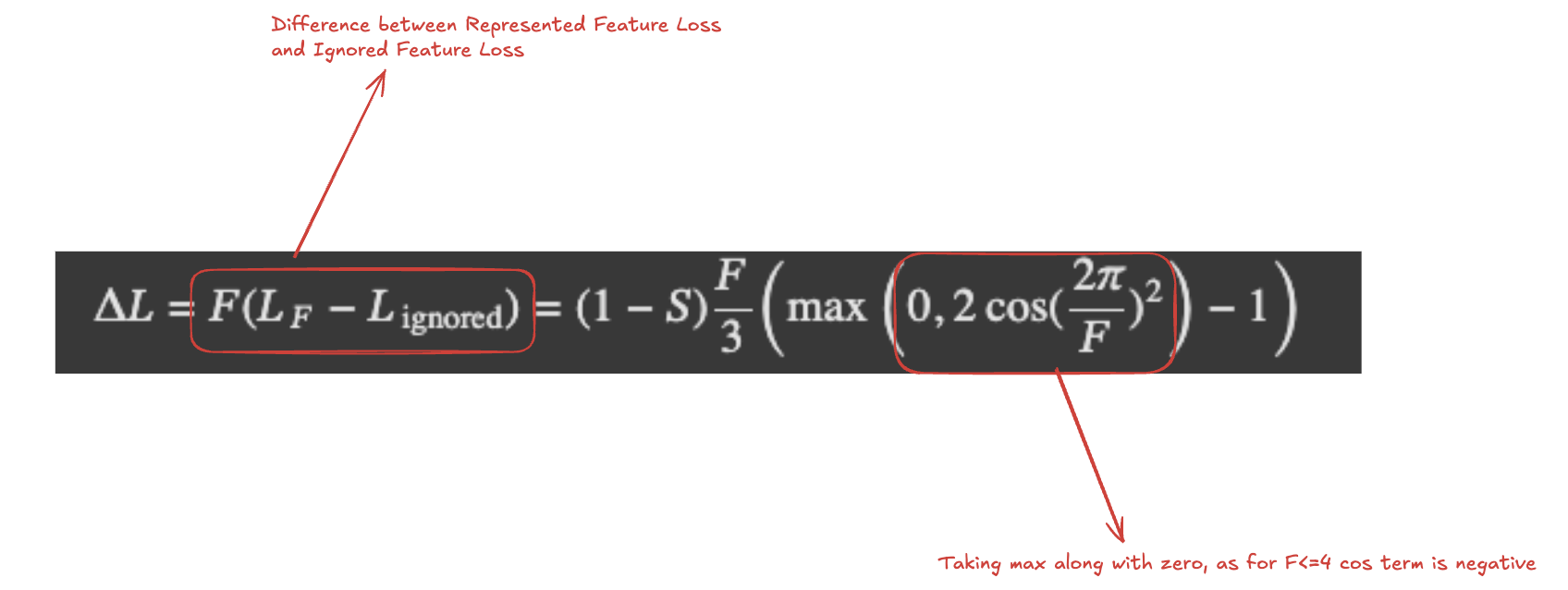
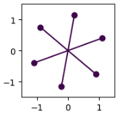
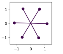
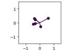
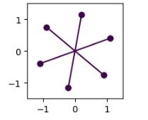
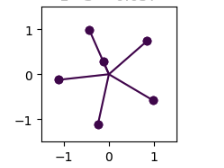
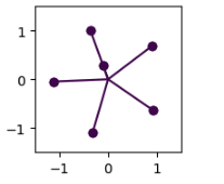
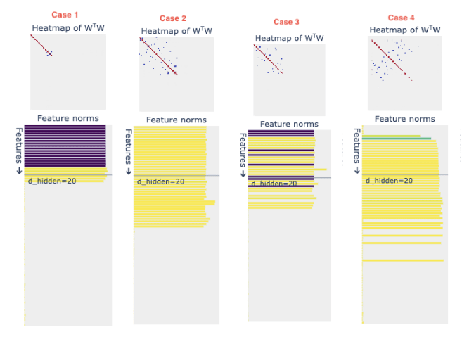
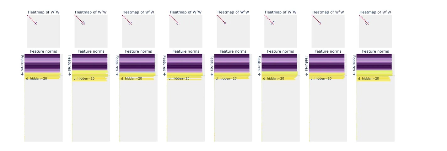
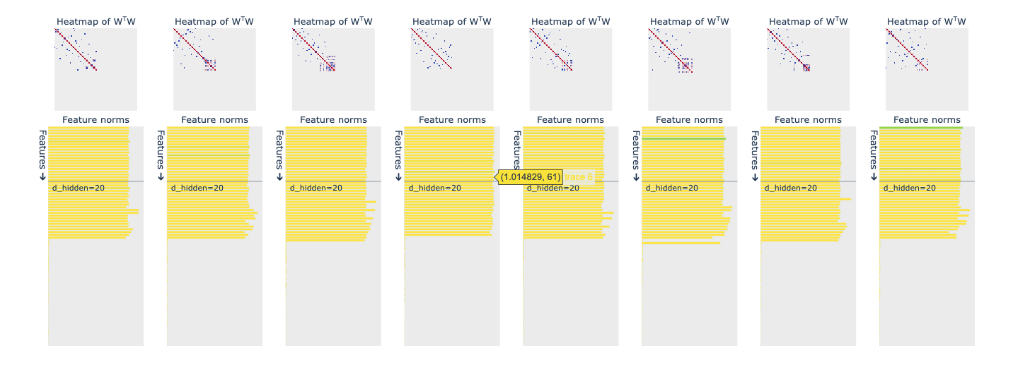
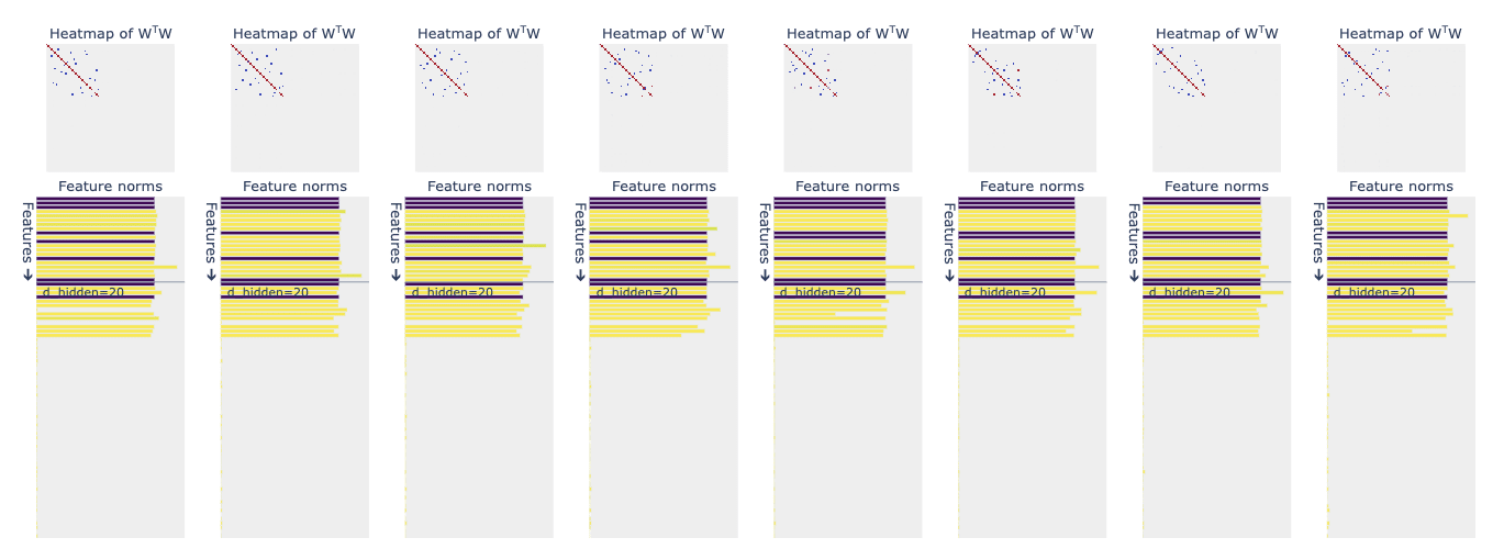
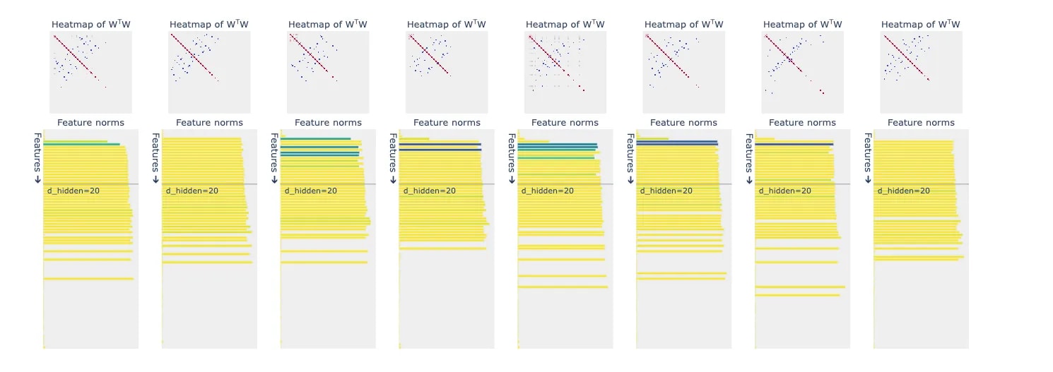
First Paper I’ve chosen is a paper named Mechanistic?. It talks about the origins of Mechanistic Interpretability as a term, a field of research and a community. So here we go…

What Do We Really Mean by Mechanistic Interpretability?

Mechanistic Interpretability (MI) has become one of the most widely used—and most ambiguously defined—terms in modern AI interpretability research. Depending on who you ask, it can mean anything from causal reverse-engineering of neural networks to simply visualizing activations. This ambiguity is not accidental; it is the product of overlapping definitions, disciplinary histories, and community-driven norms. In this post, I unpack where this confusion comes from, how MI differs (and overlaps) with NLP Interpretability (NLPI), and why these tensions matter for the future of the field.

Four (and a Half) Definitions of Mechanistic Interpretability

The term mechanistic interpretability is currently overloaded. At least four distinct definitions circulate in the literature and community discourse:

1. Narrow technical definition: A research program focused on understanding neural networks through their causal mechanisms.
2. Broad technical definition: Any work that studies model internals—weights, activations, attention patterns, or intermediate representations.
3. Narrow cultural definition: Research originating from the MI community, historically associated with forums like Distill, LessWrong, or the AI Alignment Forum.
4. Broad cultural definition: Interpretability research in AI at large, especially in language models.
5. Author-based definition (implicit): Compounding the confusion, “mechanistic interpretability” is sometimes used to describe who wrote a paper rather than what methods or goals it involves.

This definitional sprawl has diluted the original meaning of MI, particularly its grounding in causality.

Mechanisms, Causality, and Abstraction

Mechanistic interpretability derives its name from causal mechanisms. A causal mechanism can be understood as a lawful transformation: a function that maps some subset of model variables (causes) to another subset (effects).

In neural networks, MI aims to discover the mechanisms that produce specific outputs from specific inputs, using intermediate representations as the primary level of abstraction.

However, real-world causal systems—biological, physical, or artificial—are deeply complex. Multiple pathways can lead to the same outcome, making full causal explanations unwieldy. Human explanations are one way to manage this complexity: they distill explanations down to the most proximal or salient mechanisms.

Neural networks offer a different option. Since we are not limited to human-scale explanations, MI often relies on causal abstraction—distilling complex causal structure into interpretable, tractable forms without restricting ourselves to only the most local mechanisms.

From Distill to “Reverse Engineering Neural Networks”

The term mechanistic interpretability was coined by Chris Olah and first publicly used in posts on Distill.pub. Early work focused heavily on understanding how weights implement mechanisms, particularly in vision models.

The phrase “reverse engineering neural networks” gained popularity later, especially after the Distill team moved to Anthropic and began publishing transformer circuit threads. The term became so dominant that even the ICML 2024 MI Workshop adopted it to define its scope.

Ironically, much contemporary MI work no longer explicitly references causal mechanisms at all. Today, almost any form of internal inspection—causal or not—is often labeled “mechanistic interpretability.”

The NLPI–MI Divide

A major theme in this discussion is the tension between two communities:

• NLPI (NLP Interpretability): Active since early LSTM and RNN models, publishing primarily in ACL and related venues.
• MI (Mechanistic Interpretability): Emerging largely from computer vision and alignment-oriented communities, later pivoting to NLP.

One of the major points of tension was that, rather than building on NLPI’s extensive prior work or engaging with them, MI community started working on interpretability research independently, often reinventing earlier findings and repeating epistemological debates around:

• Correlation vs. causation
• Simple features vs. complex subnetworks
• Expressive mappings vs. constrained interpretations

This duplication was not purely technical, it was cultural.

Below discussed are some of the technical avenues where such duplication can be seen.

Vector Semantics: Old Lessons, New Names

The explosion of vector semantics after word2vec sparked extensive work on interpreting embeddings. Many modern ideas like task vectors, steering vectors, additive representation properties, trace their lineage to this era.

But early critics showed that embedding structure often reflects word frequency rather than deep semantic meaning. Many of these critiques remain highly relevant today as well, especially for correlational interpretability methods like similarity metrics and activation comparisons.

Neurons, Circuits, and Polysemanticity

Both NLPI and MI have attempted to localize concepts within models:

• NLPI localized linguistic phenomena to neurons or layers.
• MI pursued neuron-level explanations and later circuits—subgraphs of neurons responsible for specific behaviors.

Single-neuron analysis, however, has faced sustained criticism:

• Large models cannot be reduced to a sum of independent parts.
• Behavioral composition is often non-linear.
• Polysemanticity, where a neuron responds to multiple unrelated concepts, makes interpretation ambiguous.

MI community tried to solve polysemanticity, one of the example was using sparse autoencoders (SAE), which still relies on the assumption of linearity and naturally emerging sparsity, but like earlier neuron analysis methods, it requires expensive causal validation.

Probing: A Familiar Story

Probing methods originated in NLPI as a way to extract linguistic information from hidden states. They were criticized for weak baselines, and lot of times, probes were extracting more information from randomly initialized vectors than full trained networks

Modern MI work often uses linear probes to project model states into interpretable subspaces, but these approaches inherit the same limitations:

• Weak causal grounding
• Sensitivity to probe capacity
• Ambiguity about what is truly encoded vs. what the probe learns

Cultural, Not Just Methodological, Differences

During the early days, machine-learning in general was primarily attributed to computer vision research and lot of interpretability works were being done in CV only, shaping the methods NLP researchers adopted. The MI term itself was first used in CV contexts before migrating to NLP after breakthroughs like GPT-3.

The deeper divide, however, was cultural:

• MI research initially lived on blogs, forums, Slack, and Discord.
• NLPI research lived in peer-reviewed venues like ACL.

The absence of NLPI researchers from online forums was misread as disinterest, when it was largely a difference in publication norms.

When MI researchers began publishing in conferences, they faced criticism for limited engagement with prior NLPI literature. Despite this, MI rapidly attracted resources, attention, and prestige, leading many NLPI researchers to adopt MI terminology.

“Everyone Is Mechanistic Now”

Today, most interpretability researchers identify, at least loosely, with MI. Funding and visibility have accelerated this shift, but terminology alone has not unified the field.

Despite methodological overlap, differences in norms, goals, and epistemology remain.

Why This Still Matters

For all the confusion and tension it introduced, the MI community has played a major role in revitalizing interpretability research. Its energy, resources, and ambition have expanded the field’s reach.

At the same time, many MI researchers are motivated by AI alignment concerns, where the long-term value of MI is actively debated. It is possible that alignment priorities will eventually shift away from MI, taking some resources with them.

But interpretability will persist.

NLPI and MI researchers share too much in common, like scientific curiosity, social responsibility, and a commitment to understanding powerful models,for this work to disappear. As long as our models remain opaque, we will keep trying to open them up.

And in that sense, the question is not whether mechanistic interpretability survives, but what we ultimately decide it means.

In past couple of years, my way of thinking has taken a turn for bad i feel, where i feel, anything that doesn’t sound interesting to do, or requires any brain power, or a solution is known is not worth doing and I’m wasting my time in doing that. It can be some coding task, where the solution is known, I dont have to spend a lot of power in figuring it out, but I still have to implement it, but my brain starts signalling that because it is known, so its automatically boring and then i procrastinate that work till eternity, and this for an Independent Researcher, where you’re your own supervisor and accountability partner, is a pretty big nightmare.

So many times I catch myself day dreaming about the “interesting” life i’ll start leading the moment i become a full-time researcher, where i’m getting paid for doing research and i dont have to stress about money (thats a topic for different day), i’ll just be free bird in its own paradise, but I miss out on the most obvious reality that these banal tasks will still be part of my day to day and are pretty important for the final result to be shared across, and when the reality doesn’t meet your hyped up expectations, you start questioning whether if this was even worth the pain and effort, had i glamorised it too much (yes, i had), and the most existential of the lot, do i even wanted to do this in the first place or was i just interested in the idea of doing research and not the actual work.

Don’t get me wrong, when push comes to shove, I’ll definitely finish the banal tasks as well, and before the committed deadline, but it’ll definitely feel like dragging a heap of wet sack and not a piece of work which leaves you satisfied at the end of the day, which is a pretty messed up thing, cause you should feel satisfied even in completing the so called “banal” part of work, cause its important. But, that push, which only if it coming from external sources, works for me, and i’m not able to motivate myself on my own to create that push.

One obvious drawback of this way of working is that lot of times I just end up thinking / dreaming about the work instead of actually doing the work, it still feels like lot of work in my head, but in reality nothing gets done, it wastes a lot of time and then my anxiety kicks in sending me in a spiral that i dont have enough time to finish it, which in turns wastes more time… well you see where this is going. Additional fuckery, this overthinking does is that it increases the resistances for doing a particular task, for a 15 min task, you end up overthinking for 45 on how to optimize it, what pros and cons i’ll get from doing it etc etc. and in the end, that task is still not finished, some would say I’m taking this thing too seriously and I should lighten up a bit, and they are probably right, but easier said than done, cause here i feel i’m fighting my core self, who is too serious a person.

Deep down, i know i dont want to be this person, I want to be someone who doesn’t take life this seriously, doesn’t overthink things, starts doing them as soon as possible, fails at them and moves on to the improvement or next thing, in short, lives in the reality instead of his head, and i plan to work on this in 2026. I dont know how it’ll go and hopefully the post-it notes stuck on my monitor keeps me in check whenever i start spiralling.

For the past couple of years, toy models have been extensively studied in the field of mechanistic interpretability. The concept of superposition, feature geometry, and how correlated/anticorrelated/uncorrelated features arrange themselves in these situations was first studied in Toy Models itself. This is my attempt to explain the theoretical foundation on why feature geometry in the infinite data regime for a ReLU model (with hidden=2) caps at a Pentagon geometry irrespective of the number of inputs. Additionally, I analyze the deviations to hexagon geometry as well, primarily analyzing two factors, i.e., initialization and the choice of optimizer, and their impact on feature geometry.

Introduction

The ReLU output model is a toy model replication of a neural network showcasing the mapping of features (5 input features) to hidden dimensions (2 hidden dimensions) where superposition can be introduced by changing the sparsity of input features. For a set of input features $x∈R^n$ and a hidden layer vector $h∈R^m$, where $n»m$, the model is defined as follows:

This model showcases how a large set of input features can be represented in a much smaller dimensional vector in a state of superposition by increasing the sparsity of the input features (sparsity tries to replicate the real-world data distribution where certain concepts are sparsely present throughout the training set). This concept and observations were first introduced in Anthropic’s Toy Models of Superposition paper

The original experiment was done on $n=5$ input features but when I try to increase the number of input features, an interesting phenomena occurs. Given the observations of a quadrilateral with $n=4$ and a pentagon with $n=5$, as the number of features increases one would expect feature geometry to be hexagon or heptagon, but in reality, the features restrict themselves to a pentagon geometry, with balance of the features (if they are learned by the model), overlapping with the existing 5 directions as shown in the figure below.

I wanted to understand in detail why this is the case and if it can help us improve our understanding of feature geometry in neural networks.

Fig.1 n_features = 6 (left) and 7 (right)

Relevance to AI Safety

One of the biggest subfields of AI safety is Mechanistic Interpretability. In this subfield, researchers try to reverse-engineer neural network models (which are considered black boxes as their internal mechanisms are unknown) and make them more interpretable. Toy model setup is a very important part of this subfield, as it allows us to do controlled experiments and understand the impact of different factors on different phenomena.

For example, the concept of superposition was first studied in Toy models of Superposition paper, which led to the creation of Sparse AutoEncoders (SAEs). Today, SAEs are an integral part of understanding the types of features a model is learning.

By understanding feature geometries in toy models, we aim to develop a strong intuition about how and when features are arranged in different geometries and the types of mechanisms governing a given geometry.

Different Data Regimes and Types of Features

Before diving deep into feature geometry and the experiments, I would like to explain the concept of data regimes because that majorly impacts the type of features the model learns.

The amount of data used to train the model has a massive impact on the types of features the model learns. Superposition, Memorization, and Double Descent showcase the impact of data regimes and how the model memorizes the dataset as features in low data regimes but transitions to learning generalizable features as the amount of data increases.

Fig.2 Increase in the data size leads to features transitioning from data features to generalizing features and the geometry converges to a pentagon. Source: https://transformer-circuits.pub/2023/toy-double-descent/index.html

I’ll be focusing on the infinite data regimes as it represents the closest condition to real-world models due to the sheer size of the datasets they are trained on. With the increase in data size, the feature geometry transitions towards the pentagon geometry, while in lower data regimes, the number of features represented was much higher due to the model memorizing the dataset.

Theoretical Intuition behind Pentagon Geometry

For building the theoretical intuition for why pentagon geometry is preferred by models, I’ll be walking you through this notebook shared by Anthropic. (Credits to Tom Henighan for open-sourcing this explanation)

The key factors governing the feature geometry is the balance between the overall loss of ignored features and the loss of represented features, along with the number of features that are ignored vs represented.

The expected loss due to ignoring a single feature can be defined as:

Fig.3 Expected loss due to ignoring a single feature

Note: A sparse regime is consiered for this scenario, as only sparse features are represented in superposition and $S$ represents the probability of $x_i$ being 0 otherwise it takes a value uniformly sampled between 0 and 1.

While the predicted value of $x_i’$ (when the feature is not ignored) can be defined by:

Fig.4 Predicted value when the feature is not ignored

The formula represents the predicted value in the form of the original input value and then bakes in the influence of nearest neighbouring features (if it is positive interference or negative interference). $mod F$ term helps us wrap around the features around every $F$ positions and $(i \pm 1 \mod F)$ refer to the nearest neighbours represented feature index.

After putting the above predicted term formula in the MSE loss formula, the loss due to the represented features can be defined by:

Fig.5 Loss due to the represented features

Currently, there are two Loss terms, and based on number of features represented, these two loss terms will be pulling the overall loss in opposite directions. Loss due to represented features will increase with the increase in the number of represented features due to increased interference from neighbouring features, but we want to avoid the Loss due to ignored features as well. So, the final entity to be minimised is the difference between $L_F$ and $L_{\text{ignored}}$ i.e.

Fig.6 Difference between $L_F$ and $L_{\text{ignored}}$

After optimizing for $\Delta L$, the optimal point of lowest loss is reached at $F=5$.

The above derivation makes some assumptions for simplification and due to that the pentagon geometry is not always followed. There are some instances when a hexagon geometry (as shown in Fig 6) is observed as well. I’ll be conducting experiments to understand more about why this geometry was observed, what factors govern it and what is fundamentally different about hexagon geometry w.r.t pentagon geometry.

Fig.7 Hexagon Geometry in Toy models

Experiments

My experiment setup is similar to the Anthropic’s Toy models of Superposition setup with some modifications of my own. The number of input features will be 6 and all of them will have equal feature importance. I’ll be considering a sparsity value of 0.057 (as this sparsity was low enough to exhibit superposition but not low enough that features are not getting learned due to data unavailability) and will be analysing the effects of Initialization and the choice of Optimizer on hexagon feature geometry and superposition in general.

Impact of Initialization

While iterating the experiments through multiple different seeds, there are multiple instances where the final geometry is a hexagon while others are a pentagon. Following are the lists of experiments I performed to understand this behaviour

Feature Norms

At the start, when I compare the feature norms, there is a striking difference in the first glance itself. The overall norm in the hexagon geometry crosses the theoretical limit of $\sqrt{5}$ and stretches to 3 while the one for pentagon plateaus at 2.5.

Fig.8 Feature Norms Pentagon vs Hexagon

Per Feature Gradient Norms and Losses

As a next step, I analyzed the trajectory of the per-feature gradient norm (to understand the types of gradient updates taking place) and compared it with per-feature loss to learn how the features are being learned.

In the case of pentagon geometry, the gradient updates for two features (dark blue and red) start at a very low point and stay low throughout the training run while for others it decreases in the later stages of the training process.

When compared against the per-feature losses, I observe that one feature is starting from a point of very low loss (very near to the optimal point) so it doesn’t need big gradient updates, but the other one is starting from a very high loss (very far from the optimal point) and still has low gradient updates indicating that its stuck in a saddle point and is unable to escape.

Fig.9 Per Feature Gradient Norm for Pentagon Seed

Fig.10 Per Feature Loss for Pentagon Seed

In the similar plots for hexagon geometry, it shows that the gradient updates decreases for all the features and the losses for all the features converge to a optimal minima as well.

Fig.11 Per Feature Gradient Norm for Hexagon Seed

Fig.12 Per Feature Loss for Hexagon Seed

This analysis indicates the effect of initialization on the starting point of features in the coordinate space and how it affects the resulting feature geometry. To properly validate the hypothesis, I performed one more experiment of patching the initialization.

Hexagon Patching

I took the initial weights of the pentagon seed and replaced the weights of only the feature that is not learnt with initialization weights of the same feature from the hexagon seed. When the model is trained with this modified initial weight matrix, the resulting geometry showcases features arranged in a hexagon geometry after weight patching v/s in a pentagon geometry before patching.

Fig.13 Unpatched Pentagon Geometry (left) and Patched Hexagon Geometry (right)

Impact of Optimizer

Secondly, I try to analyze the impact of the optimizer on the feature geometry. In this experiment, I chose 4 types of optimizers namely SGD, RMSProp, Adam, and AdamW.

In the experiments, SGD underperformed in all cases leading to non-superimposed and unlearned features irrespective of hyperparameters. For RMSProp, Adam & AdamW, all of them exhibit superposition and the resulting feature geometry was a delicate balance between initialization and choice of optimizer. Not all optimizers will give hexagon geometries at the same seed but once carefully chosen, the combination of the right seed and right optimizer will lead to the hexagon geometry, otherwise, it exhibits pentagon geometry.

Fig.14 SGD (first), Adam (Second), AdamW (Third), RMSProp (Fourth)

Conclusion

In this analysis, I try to understand the core intuition behind the feature geometry in toy models with hidden dimension=2 and assumptions behind it. I also try to understand in what cases the experimental results deviate from the theoretical foundation leading to a hexagonal geometry and analyse the impact of Initialization and Optimizer on the resulting feature geometry.

Limitations and Future Work

While I found some pretty interesting results, there is still a much deeper analysis which can be conducted to study hexagon geometry and why it occurs. Also, this analysis was done on toy models so will the findings scale to bigger models or not, thats yet to be seen.

Acknowledgement

I want to thank Bluedot Impact for organizing the AISF Alignment Cohort. Past 12 weeks have been really valuable in improving my understanding on Mechanistic Interpretability and AI Safety in general.

Additionally, I want to thank Shivam Raval for guiding me through the research process.

About Me

Hey, I’m Shreyans and I’m an Independent Interpretability Researcher based out of Bengaluru, India. After 8 years of working in the Applied ML field, I finally took the leap of faith to take a small career break to pursue my interest of Interpretability Research. This work is my capstone project as part of the AISF Alignment Cohort by Bluedot Impact. If you have any questions or feedback on this blog, feel free to reach out to me on jshrey8@gmail.com or any of my socials in my profile. I hope I was able to improve your understanding on feature geometry in toy models. Cheers!!

Abstract

This post summarises my findings on the effects of Non-Uniform feature sparsity on Superposition in the ReLU output model, introduced in the Toy Models of Superposition paper, the ReLU output model is a toy model which is shown to exhibit features in superposition instead of a dedicated dimension (‘individual neuron’) devoted to a single feature. That experiment showed how superposition is introduced in a model by varying the feature sparsity values. However, a uniform sparsity across all the features was considered to keep things interpretable and simple. This post explores the effects of non-uniform sparsity on superposition for a similar experiment setup.

This question was listed in Neel Nanda’s 200 Concrete Open Problems in Mechanistic Interpretability post. I’ve been interested in AI Interpretability for a long time but wasn’t sure how to enter the field. I discovered the field of mech-interp recently when I was working on some other project and instantly felt connected to the field. This is my first post on LW and this project is my attempt to increase my comfort working with mech-interp problems and build the necessary reasoning for solving more complex problems.

Introduction

The ReLU output model is a toy model replication of a neural network showcasing the mapping of features (5 input features) to hidden dimensions (2 hidden dimensions) where superposition can be introduced by changing the sparsity of input features. For a set of input features x∈Rn and a hidden layer vector h∈Rm, where n»m, the model is defined as follows:

This model showcases how a large set of input features can be represented in a much smaller dimensional vector in a state of superposition by increasing the sparsity of the input features (sparsity tries to replicate the real-world data distribution where certain concepts are sparsely present throughout the training set). This concept and observations were first introduced in Anthropic’s Toy Models of Superposition paper

Before we go ahead with the analysis, let me give you a primer on some important terms we will encounter in this post:

• Feature Importance: Feature importance can be defined as how useful a particular feature is for achieving lower loss. It’s augmented in the ReLU model loss as a coefficient on the weighted mean squared error between the input and the output. $L=∑_x∑_iI_i(x_i−x^′_i)^2$ where $I_i$ is the importance of the feature $i$
• Feature Sparsity: Feature sparsity is defined by how frequently a feature is present in the input data. In the ReLU Output model, its defined as the probability of the corresponding element in x being zero. An alternate quantity called Feature Probability defined as 1 minus Sparsity is also used in this formulation.

To summarise the paper’s findings, it showcases that as we increase the sparsity of input features, more features start getting represented in superposition. When sparsity is high, features of higher importance are represented as a dedicated dimension in the hidden layer, but as we increase the sparsity, lower-importance features start getting represented along with higher-importance features in superposition.

In the below figures, as we move from left to right, feature sparsity is gradually increased showcasing the transition of how more and more features start getting represented in superposition.

As we increase the feature sparsity from left to right, number of features represented by the hidden layer increases. Yellow represents the feature with highest importance and as we go more green, feature importance decreases

Dark colors in the second figure mean feature is represented as a dedicated dimension and as the color transitions to yellow, it indicates feature being in superposition (Source: https://transformer-circuits.pub/2022/toy_model/index.html#demonstrating-basic-results)

I attempt to extend that representation one step further by considering a non-uniform sparsity instead of a uniform sparsity for input features as not all concepts are equally sparse in a training dataset.

Experiment Setup

In my experiment setup, I’m considering two main levers, namely Feature Sparsity and Feature Importance. As we are considering non-uniform sparsity, its combined effect with feature importance plays an important role in the final result and leads to some interesting findings. To showcase different situations, I’m considering four different scenarios:

1. Feature with the highest importance has the least sparsity and as we go down feature importance, the sparsity increases
2. Feature with the highest importance has the highest sparsity and as we go down feature importance, the sparsity decreases
3. Random feature sparsity across features
4. Constant feature importance and increasing feature sparsity (similar to Case 1.)

Also, to see the effect of random seed on the final results, every scenario was running eight instances while keeping everything constant.

Note: Similar figures that you will encounter from this point onwards has a slightly different interpretation. All the eight instances in every case have the same distribution of feature sparsity. They are to be interpreted as outputs of different random seeds while every other hyperparameter is kept constant. Feature sparsity is not decreasing as we move from left to right (unlike the preceding figures) in the following figures.

Results

No of Features Represented

In all the scenarios considered with non-uniform sparsity, never once are all the five input features represented in the hidden layer (as we saw in the case of uniform sparsity). No. of feature represented maxes out at 4 and hovers around 3 in a lot of scenarios. The below figure illustrates the phenomena for Case 1, for a detailed view of figures from all the scenarios, refer to this page.

Case 1: Feature with the highest importance (in yellow) has the least sparsity and as we go down feature importance (color gets greener), the sparsity increases

Does this mean that in the case of non-uniform sparsity, all the features will never be represented in the hidden layer and we will always lose some concepts?

To validate this from a different direction, I tried analyzing the number of features represented in a higher hidden dimension (h = 20, no of input features = 80). To estimate the amount of features represented in the hidden layer, I’m choosing the Frobenius Norm as a proxy. The table below summarises the Frobenium Norm values for all the scenarios considered:

We can see, that the Frobenium Norm value in the case of Uniform Sparsity is the highest when compared to all the cases of Non-Uniform Sparsity which indicates the number of features represented when sparsity is uniform will most likely always be higher than when compared to non-uniform sparsity.

Effects on Superposition

Superposition comparison between different cases considered. Purple color indicates features in dedicated dimension, green indicates feature in superposition with less interference, yellow indicates features in superposition with more interference. Blank indicates features not represented in hidden layer.

In Case 1, we see the lowest feature representation and the least amount of superposition (showcased in yellow) which was an expected outcome as we are assigning the least amount of sparsity to the most important features. The blanks in the below figure indicate a particular feature is not represented at all in the hidden layer.

Case 1: showcasing more important features getting dedicated dimensions (in purple), while lower importance features are in superposition (in yellow). Blanks indicates features not represented in the hidden layer.

Case 2 was pretty interesting as we noticed that all the features represented are always in superposition and none of the features is ever represented as a dedicated dimension irrespective of feature importance.

Case 2: showcasing all the features (in yellow) in superpositon. Blanks indicates features not represented in the hidden layer.

Case 3 is the closest we come to a real-world scenario, where feature sparsity is distributed randomly across features, irrespective of their importance. It looks like an averaged-out scenario of Cases 1 & 2 and strikes an approx. midpoint between dedicated dimensions vs superposition when representing features.

What exact combination of feature sparsity and feature importance governs this behaviour is something I wasn’t able to answer in my analysis and I think it’ll be an important question to answer as it can help us interpret the feature representations in real-world models.

Case 3: Some features are represented as dedicated dimension (in purple) and some are in superposition (in yellow)

To check a clear effect of sparsity on superposition, we consider Case 4 where we keep the feature importance constant and consider an increasing sparsity (similar to Case 1.)[1]

In this case, we stumble on a weird observation where the few features with the least sparsity are not even learned and represented in the hidden layer. The representation starts after a couple of features where all of the represented features (barring a few exceptions due to random seed) are in superposition all the time.

Case 4: Constant feature importance with increasing sparsity (as we go from top to bottom). Darker color (Green or dark blue) indicates less interference from other features meaning the feature is somewhat in superposition but to a lesser extent compared to features in yellow.

Presently, I don’t have a clear intuition on why this is the case but this is quite a contrary observation compared to my expectation.

Additionally, this scenario also gives us an intuition that feature importance has a bigger contribution in deciding whether a feature is represented as a dedicated dimension or not when compared to sparsity.

Just to give you some background, I’m a civil engineering graduate without any foundational CS, math or statistics knowledge and have been working as an Applied Data Scientist for the past 8 years. As of 2024, I’ve been interested in AI safety and ethics research for the past 3 years and really want to crack into it. So in a nutshell, for all my professional life, I’ve been playing catchup with whatever I’ve wanted to do. Initially, it was with ML fundamentals and trying to learn as much variety as possible, be it forecasting, recommender systems, search, deep learning, reinforcement learning, YOU JUST NAME IT!! If it involved math and CS somehow, I would be interested in that. Never once, did I felt like sitting comfortably wherever I was and just enjoy life.

So an obvious by-product of all this juggling was a constant comparison with other folks present in the field and obviously (me being me!! 😕), the comparison was with accomplished folks in the field who have been working in that niche for multiple years (in other words, WAY MORE TIME THAN ME!!). I always had this urge to be able to learn all the tricks of that trade immediately and just master that niche.

During all the comparative analysis I did to determine how I could reduce the gap between me and others (while obviously ignoring the obvious ones 🤪), I just put my foot on the gas pedal and was at it studying or working on projects, but at the end of the day, it never felt like I was doing enough to catch up, and whenever I compared again with others, I was always on a backfoot. This idea got ingrained in me so much that I almost believed that their systems were optimized to unreal extents in terms of productivity, focus and yield and to chase that I literally gave up on my hobbies and all kinds of entertainment (read as “rest” or “break”) but that feeling never went away.

My mind wasn’t far behind in playing games either, it always moved benchmarks and goalposts while doing any kind of comparison, just so that I could arrive at the conclusion that I’m not doing enough!!

I still struggle with this idea to this day and there are days I spiral like the bestest lattu you’ve ever seen in your life. But slowly I’m getting to terms with the realisation that there is a high probability if you are asking yourself this question, YOU ARE DOING ENOUGH!!! already. The fact you are introspecting and trying to better yourself indicates that you have already explored lots of ideas and you are on the right path.

In the end, I would just recommend one thing, don’t give up on your hobbies and fun projects, they make you a complete and interesting human being, because on the work side YOU ARE ALREADY DOING ENOUGH!!.